How to fix Pivot Table Field Name is not Valid error in Excel?

The Pivot Table field name is not valid error can occur while creating, modifying, or refreshing data fields in the pivot table. It can also appear when using VBA code to modify the pivot table. It usually occurs when there is an issue with the field name in a code or if there is a hidden or empty column in the pivot table. However, there could be many other reasons behind this error.

Why the “Pivot Table Field Name is not Valid” Error Occurs?

You can get the “Pivot Table field name not valid” error in Excel due to several reasons. Some possible causes are:

• Excel file is corrupted
• Damaged fields in the pivot table
• Pivot table is corrupted/damaged
• Hidden columns in the pivot table
• Macro (referring to the pivot table) is corrupted
• Preserve formatting option is enabled
• Missing or incorrect fields in the VBA code
• Issue with workbook.RefreshAll method syntax (if using)
• Pivot Table contains empty columns
• Header values or header column is missing in the Pivot Table
• Pivot table is created without headers
• Columns/rows are deleted from the Pivot Table

Methods to Fix Pivot Table Field Name is not Valid Error in Excel

You can get this error if you have selected the complete data sheet and then trying to create the Pivot Table. Make sure you choose only the data fields that you want to insert in the Pivot Table. If this is not the case, then follow the troubleshooting methods mentioned below.

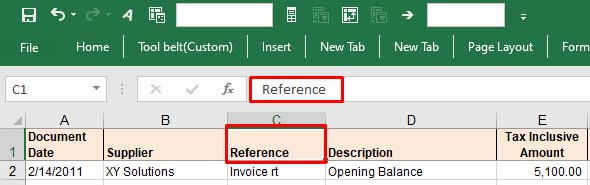
Method 1: Check the Header Value in the Pivot Table

The “Pivot table field name is not valid” error can occur if you have not set up the pivot table correctly. All the columns having data in them should have header and header values. A pivot table without a header value can create issues. You can check the header and its value from the Formula bar. Change the header if the header value is too lengthy or if it contains special characters.

Method 2: Check and Change the Data Range in the Pivot Table

The “Pivot Table field name is not valid” can occur while modifying a field in Pivot Table. It usually occurs if you’re trying to add or modify the field by selecting an incorrect data range in the Create PivotTable dialog box. The “Create PivotTable“ feature helps define how data would be displayed within the pivot table.

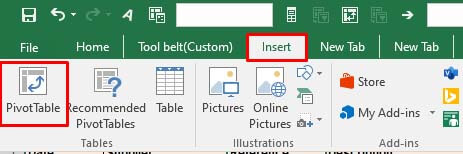
Let’s take a scenario to understand this. Open the Excel file with PivotTable. Click on the fields (you want to add), go to the Insert option, and click PivotTable.

If you select an incorrect range, i.e. A1:E18, instead of correct range - “Expenses**!$A$3:Expenses!$A$4**,” you will immediately get the error message.

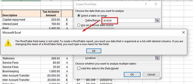
So, type the correct range under the Select a table or range option and click OK.

Method 3: Unhide Excel Columns/Rows

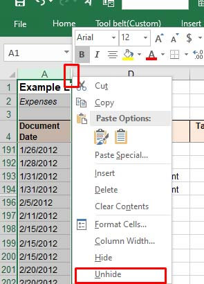
The error can also occur if some columns/rows of the Pivot Table’s data source are hidden. When you try to add a hidden column as a field in the PivotTable, the Excel application will fail to read the data of the hidden column. You can check and unhide the Excel columns by following these steps:

• Open the Excel file.

• Locate the hidden column number.

• Move your cursor on the hidden column number and right-click on the space between the columns. Click Unhide.

  

Method 4: Check and Delete Empty Excel Columns

Sometimes, you can get the “Pivot Table field name is not valid” error if you are trying to use an empty column as a field in your Pivot Table. Check the columns with no values in all cells. If found, then delete the empty columns. This method is ideal for small-size Excel files. However, for large-sized files, it is a time-consuming process.

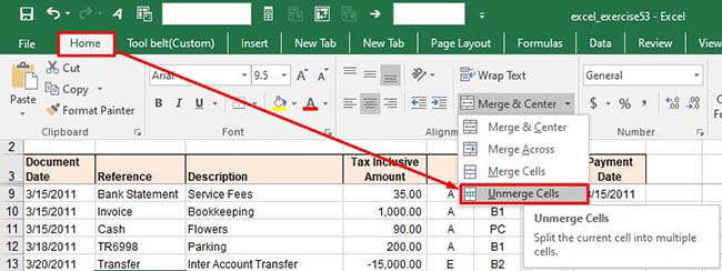
Method 5: Unmerge the Column Header (If Merged)

The “Pivot Table field name is not valid” error can also occur due to merged column headers. The pivot table references headers to identify the data inside the rows or columns. The merged headers can sometimes create data inconsistencies. You can try unmerging the column headers to fix the issue. Follow these steps:

• In the Excel file, go to the Home

• Click the Merge & Center option and select Unmerge Cells from the dropdown.

  

Method 6: Disable the Background Refresh Option

If the “background refresh” option in the Excel file is enabled, it may also create issues with Pivot Table. The Excel updates all the pivot tables in the background even after a small change if the background refresh option is enabled. This may create issues if the Excel file is large with too many tables. You can try turning off the “background refresh” option in the Excel file to troubleshoot the issue. Here is how to do so:

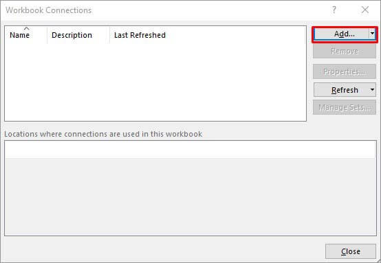
• In the Excel file, go to the Data tab and then click Connections.

  

• In the Workbook Connectionsdialog box, click on the ‘Add’ dropdown to add the workbook (in which you need to modify the refresh settings).

  

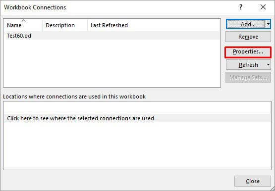
• Once you have chosen the Excel file, click Properties.

  

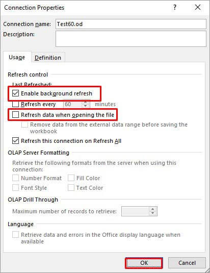
• In the Connection Properties window, unselect the **”Enable background refresh”**option, select the “Refresh data when opening the file“, and click **OK.

  

  **

Method 7: Check the VBA Code

The error can also occur when working with PivotTable using VBA code in Excel. Some Excel users reported this error on forums as run-time error 1004: The PivotTable field name is not valid. This error usually occurs when there are issues in the VBA code, affecting the PivotTable data source or field references. You can check field names referring to PivotTable or Workbook.RefreshAll function syntax and other errors in the code.

Method 8: Repair your Excel File

One of the reasons behind the “Pivot Table field name is not valid” error is corruption in the Excel file, containing the Pivot Table. You can repair your Excel file using Microsoft built-in utility - Open and Repair. Here’s how to use this utility:

• In Excel, navigate to File > Open.

• Click Browse to choose the affected workbook.

• The Open dialog box will appear. Click on the corrupted file.

• Click the arrow next to the Openbutton and then select Open and Repair.

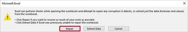
• You will see a dialog box with three buttons - Repair, Extract Data, and Cancel.

  

• Click on the Repair button to recover as much of the data as possible.

• After repair, a message is displayed. Click Close.

Method 9: Use a Professional Excel Repair Tool

If the Excel file is heavily damaged or corrupted, then the “Open and Repair” utility may not work or provide the intended results. In such a case, you can opt for a professional Excel repair tool. Stellar Repair for Excel is an advanced Excel file repair tool, which is highly recommended by experts. It can repair severely corrupted Excel files and restore all the data from corrupt file, including pivot tables. This tool comes with a user-friendly interface that even a non-technical user can use. You can try the software’s demo version to check how it works. The software is fully compatible with all Excel versions, including Excel 2019.

Conclusion

The Excel error “Pivot Table field name is not valid” can occur due to hidden or merged column/row headers, empty columns/rows, corrupted pivot table, and various other reasons. You can try the methods mentioned above to fix the error. If this error has occurred due to corruption in the Excel file, then you can use Stellar Repair for Excel - an advanced tool to repair corrupted pivot table, macros, fields, or other elements in an Excel file. It is compatible with all Windows editions, including the latest Windows 11. It can help fix the error if the data source or Pivot table configuration is affected by corruption.

Get Rid of corrupt Excel File

Summary: What to do when an Excel file is corrupted? This is a common question that is often asked by Microsoft Excel users. If you too are seeking an answer to this question, read the blog to learn about a few manual workarounds and a specialized Excel file repair tool to resolve the Excel file corruption issue.

An Excel file gets corrupted due to various reasons such as a virus/malware attack, sudden system shutdown when the Excel file is still open, power failure while working with an Excel spreadsheet, etc.

When Microsoft Excel detects corruption in a workbook, it attempts to repair the workbook by starting ‘File Recovery mode’.

Tip! If the file recovery mode doesn’t start, you may use the manual repair process or an Excel repair tool, such as Stellar Repair for Excel to repair a corrupted Excel file. The software can help you quickly retrieve contents from a damaged, corrupt, or inaccessible Excel file and restore the file to its original state.

There even exist a few manual tips that can be used to recover data from damaged MS Office Excel files.

Workarounds to Use When an Excel File is Corrupted

Note: Before carrying out any of the repair and recovery workarounds, it is advised that you must save a backup copy of the damaged file. This is to prevent your files from turning completely inaccessible in case the methods fail to give desired results.

Workaround 1: Use the Open and Repair Method

If MS Excel cannot repair a corrupted workbook automatically, you can try to do it manually. To do so, perform the following:

• Open the corrupt file, like you normally open any file, by clicking File > Open.
• Browse and locate the folder containing the corrupted document.
• When the Open dialog box is displayed:
• Select the Excel document.
• Click on the arrow present to the right side of the Open button and select Open and Repair option.

Figure 1 – Open and Repair Feature

If this doesn’t help repair the broken Excel file or you encounter  Open and Repair does not work issue, proceed with the next workaround.

Tip! Try an alternative solution, i.e. Stellar Repair for Excel software to repair and recover corrupt Excel files (.xlsx or .xls) when the ‘Open and Repair’ method won’t work.  

Workaround 2: Restore an Excel File with a Shadow Copy

If you’re a Windows 7 or Vista user, you can try restoring the corrupted spreadsheet by using a shadow copy (or a previous version). [Shadow copy](https://en.wikipedia.org/wiki/Shadow_Copy#:~:text=Shadow%20Copy%20(also%20known%20as,the%20Volume%20Shadow%20Copy%20service .) is basically a snapshot (backup copy) of computer files or volumes. The snapshot may contain an older version of your Excel file that has become damaged now. To find out, do the following:

• Launch File Explorer, and right-click the folder in which the file is saved.
• Choose Properties.
• Look for and click the Previous Versions tab. This will display a list of entries under Folder versions or File versions, going back a few days or weeks.
• Double-click one with a date when the file was accessible and could be read. Then, try to open its older version. If it opens, save the older version with a new name and execute the procedure with new file/folder entries.

Figure 2 – Volume Shadow Copy

You would have to repeat the process until you reach the point where the file became damaged. With this, you will get a baseline version of the file, but data may still have been lost.

Workaround 3: Test your Assumptions

If you receive a message saying “Excel file corrupted and cannot be opened”, you would probably believe it. However, there could be other reasons besides corruption that may cause Excel to throw this error message.

Your Office suite, which Excel is a part of, maybe having some primary issues in it causing problems while opening one Excel document. So, try opening another Excel file to check if the problem exists with all the files or just one.

If other Excel documents work correctly, it means that only the particular document is corrupt. On the contrary, if the issue is with your Office suite, repairing the current Office installation may help fix the issue. For this, perform these steps:

• Go to Control Panel and click Uninstall the Program.
• Choose Office.
• Click Change, and hit the Repair button.

You can reinstall the entire Office package. Once reinstalled, try to open the file to check if the issue has been fixed and the Excel file repaired.

Figure 3 – MS Office Repair

Workaround 4: Use Excel File Repair Tool

If the above manual solutions fail, use Excel repair software to successfully repair your damaged Excel workbook and recover all its data. Essentially, the software rebuilds damaged Excel workbook data at a granular level to recover every single object & all the original properties of the workbook.

Suggested Read: How to repair corrupt Excel files using Stellar Repair for Excel?

Why Use Stellar Repair for Excel Software?

• Repairs severely corrupted XLSX and XLS files.
• Can handle corrupt Excel files of any size.
• Demo version allows previewing recoverable Excel file items for free.
• Supports Microsoft Excel 2019 and all lower versions.
• Compatible with Windows 10 and lower versions.
• Tested and recommended by Microsoft Excel MVPs.

Final Word

When an Excel file is corrupted, it won’t open at all or you won’t be able to access all the file data. Such a situation can lead to unnecessary halts, impacting work productivity.

There are manual workarounds that may help fix the corrupt Excel file and recover its data, such as the ones covered in this blog. However, these solutions might not work in severe corruption cases and may require technical assistance. Also, they may result in some data loss.

To overcome the limitations of manual workarounds, it is recommended to go for a professional Excel file repair tool such as Stellar Repair for Excel . It helps repair corrupt Excel (XLS or XLSX) files and restores all worksheet data, such as the table, chart, chart sheet, cell comment, sort and filter, image, formula, etc. in a few simple clicks. Moreover, the software provides a free preview of the recoverable data with its demo version. You can check the preview to evaluate how the software works.

Quick Fixes to Repair Microsoft Excel 2013/2016 Content related error

Summary: The blog outlines some quick tips to fix ‘We found a problem with some content’ error in Microsoft Excel 2013/2016. It explains manual procedure to resolve the error and also suggests an automated tool to perform the repair process to retrieve all possible data from a corrupt workbook.

Sometimes, when opening an MS Excel file, you may receive an error message that reads:

“**We found a problem with some content in ‘filename.xlsx’. Do you want us to try to recover as much as we can? If you trust the source of this workbook, click Yes.**“

Figure 1 – Excel ‘found a problem with some content’ Error Message

What Causes ‘We Found a Problem with Some Content’ Error?

There is no clear answer as to what results in the Excel error – ‘**We found a problem with some content in <filename.xlsx>**’. However, based on some user experiences, it appears that the error occurs due to corruption in an Excel workbook. It may turn corrupt when:

• You try opening the Excel file saved on a network-shared drive.
• A string is added in a cell in Excel, instead of a numeric value.
• Text values in formulas exceed 255 characters.

How to Resolve ‘We Found a Problem with Some Content’ Error?

Follow these tips to fix the Excel error:

IMPORTANT! Before you follow the tips to resolve the Excel error, keep these points in mind: Make sure you have closed all of the opened Excel workbooks. Try restoring Excel file data from the most recent backup copy. If you don’t have a backup copy, make a copy of the corrupt Excel file and perform repair and recovery procedures on that backup copy.

Tip #1: Repair Corrupt Excel File

File Recovery mode is a native Excel recovery utility that automatically opens whenever any inconsistencies are found in the worksheet. If Microsoft doesn’t detect any issue or fails to open the File Recovery mode, you can start it manually to recover the corrupt Excel file. To do so, follow the steps below:

1. Click on the File menu, and then select Open.
2. In the Open dialog box, navigate to the folder location where the corrupt Excel file is saved.
3. Select the corrupt file, and then click on arrow sign available next to Open button to select Open and Repair option.

Figure 2 – Open and Repair Feature in Excel

1. Next, click Repair to recover maximum possible data.
2. If the repair is not able to recover the data from the workbook, select Extract Data to extract all possible formulas and values from the workbook.

If repairing the corrupt Excel file doesn’t work, you can try an Excel file repair tool to fix corruption errors. You can also try to recover data from the corrupt file manually by following the next tips.

Read this: What to do when Open and Repair doesn’t work?

Tip #2: Set Calculation Option to Manual

To make the file accessible, try setting the calculation option in Excel from automatic to manual. As a result, the workbook will not be recalculated and may open in Excel. For this, perform the following:

1. Click File, and then click New.
2. Under New, click the Blank workbook option.
3. When a blank workbook opens, click File > Options.
4. Under the Formulas category, pick Manual in the Calculation options section, and then click OK.

Figure 3 – Select Manual in Calculation options

1. Now, again click on the File menu and then click Open.
2. Navigate to the corrupt workbook, and double-click it.

When the workbook opens, check if it contains all the data. If not, proceed to the next tip.

Tip #3: Copy Excel Workbook Contents to a New Workbook

Several users have reported that they were able to fix ‘We found a problem with some content in ’ error message by copying contents from the corrupt workbook to a separate workbook. Detailed steps are as follows:

1. Open the Excel workbook in ‘read-only’ mode, and copy all its contents.
2. Create a blank new workbook and paste the copied contents from the corrupt file to the new file.

Tip #4: Use External References to Link to the Damaged Workbook

Use external references to link to the corrupted workbook. By implementing this fix, data contents can be retrieved. However, it is not feasible to recover formulas or calculated values using this solution.

Follow the steps below:

1. In Excel 2013/2016, click File > Open.
2. Navigate to the folder where the corrupt file is saved.
3. Right click the file, select Copy, and then click on Cancel.
4. Again, click on File and then New.
5. Under New option, click on Blank workbook.
6. In the cell A1 of new workbook, type =File Name!A1 (where File Name indicates the name of the damaged workbook being copied in Step 3).
7. If Update Values dialog box appears, click the corrupt workbook, and choose OK.
8. If Select Sheet dialog box appears, click the appropriate sheet, and then click OK.
9. Select cell A1.
10. Next, click Home, and then click Copy (or, press Ctrl +C).
11. Starting in cell A1, select area approximately the same size as that of the cell range that contains data in the damaged workbook.
12. Next, click Home and select Paste (or click Ctrl + V).
13. Keep the range of cells selected, click Home and then Copy.
14. Finally, click on Home, click on the arrow associated with Paste and under Paste Values click on Values.

This will remove the link to the corrupt workbook and will retrieve data. But, keep in mind, the recovered data will no longer contain formulas or calculated values.

Alternative Solution – Stellar Repair for Excel

If the above manual methods fail to fix the ‘We found a problem with some content in Excel error’, try using the Stellar Repair for Excel software to resolve this error. The software helps repair and recover corrupt Excel files in just a few clicks. It can be used on a Windows 10/8/7/Vista/XP/NT machine to repair a corrupted workbook and recover every single bit of data from all the versions of the Excel workbook.

Read this: How to repair corrupt Excel file using Stellar Repair for Excel?

Conclusion

In this blog, we discussed some possible reasons behind Microsoft Excel 2013/2016 ‘We found a problem with some content’ error. The error may occur when an Excel file becomes corrupt. You may try repairing the corrupted Excel file manually by using the built-in ‘Open and Repair’ feature. Or, try the manual workarounds to extract data from the corrupt file discussed in this post. If the manual solutions don’t work for you, using Stellar Repair for Excel can come in handy in repairing the corrupt Excel (.xls/.xlsx) file and recovering the complete file data.

[Fixed] Excel Found a Problem with One or more Formula

Summary: The error ‘Excel found a problem with one or more formula references in this worksheet’ may appear while saving the Excel workbook. It occurs when Excel found a problem with the formula used in the sheet. However, it may also occur when the Excel workbook gets damaged or corrupt. In this guide, we’ve explained the reasons that may lead to this Excel error and methods to resolve the error, by using various Excel options and a third-party Excel file repair software.

If you are experiencing the ‘Excel found a problem with one or more formula references in this worksheet’ error message in the Excel workbook, it indicates that the Excel file is corrupt or partially damaged. However, it may also occur due to incorrect reference to a wrong cell or object linking, which is not working. The complete error message says,

‘Excel found a problem with one or more formula references in this worksheet. Check that the cell references, range names, defined names, and links to other workbooks in your formulas are all correct.’

In any case, resolving the error is critical as it doesn’t let you save the file and may result in loss of information from the Excel workbook.

Reasons for Excel Formula References Error

A few reasons that may lead to such error are as follows,

• Wrong formula or reference cell
• Incorrect object linking or link embedding OLE
• Empty or no values in named or range cells
• Multiple Excel files (not common)

Methods to Resolve ‘Excel Found a Problem with One or More Formula References in this Worksheet’ Error

Following are a few methods that you can follow to fix Excel file that can’t be saved due to problems with one or more formula references in the worksheet.

Method 1: Check Formulas

If the problem has occurred in a large Excel workbook with multiple sheets, it’s quite hard to pinpoint the problem cell. In such cases, you can use the Error Checking option that runs a scan and checks for a problem with formulas used in the worksheet.

To run Error Checking in the Excel sheet, follow these steps,

• Go to Formulas and click on the ‘Error Checking’ button

• This runs a scan on the sheet and displays the issues, if any. If no issue is found, it displays the following message,

The error check is completed for the entire sheet.

In such a case, you can try saving the Excel file again. If the error message persists, proceed to the next method.

Method 2: Check Individual Sheet

The problem may also occur due to an issue with one of the sheets in the workbook. To find the faulty sheet and fix the problem, you can copy each sheet content in a new Excel file and then try to save the Excel file.

This will help you find the faulty sheet from the workbook that you can review. This method makes the entire process of troubleshooting Excel formula reference error quite easy and convenient.

In case the error is not fixed, you can back up the faulty sheet content and remove it from the workbook to save the Excel file.

Method 3: Check Links

When the Excel file contains external links with errors, MS Excel may display such error messages. To check and confirm if external links are causing the error, follow these steps,

• Navigate to Data Tab > Queries & Connections > Edit Links
• Check the links. If you find any faulty link, remove it and then save the sheet

Method 4: Review Charts

You can review the charts to check if they are causing the formula reference error in Excel. It may take a while based on the size of the Excel file. Sometimes, it’s not practically possible to track down which Excel chart object is causing the error. Thus, you need to check specific locations, such as:

1. Check horizontal axis formula inside Select Data Source dialog box
2. Check Secondary Axis
3. Check linked Data Labels, Axis Labels, or Chart Title

Method 5: Check Pivot Tables

To check Pivot Tables, follow these steps,

• Navigate to PivotTable Tools > Analyze > Change Data Source > Change Data Source…

• Check if any of the formula used is problematic. Sometimes small typo, such as misplaced comma, can lead to such problems in Excel. Thus, check each formula thoroughly and correct the formulas wherever needed.

Method 6: Use Excel Repair Software

When none of the methods resolve the error, then you can rely on advanced Excel repair software , such as Stellar Repair for Excel. It’s a powerful tool that is recommended by several MVPs and IT administrators for resolving common Excel errors, such as ‘Excel found a problem with one or more formula references in this worksheet.’

It repairs corrupt or damaged Excel (.xls/.xlsx) files, recovers Pivot tables, charts, etc., and save them in a new Excel worksheet. It helps Excel users, facing formula reference error, restore their Excel file without any risk of data loss, while preserving the sheet properties and formatting with 100% precision.

Conclusion

Although the error ‘Excel found a problem with one or more formula references in this worksheet’ can be resolved by using various options in MS Excel, it may lead to a partial loss of information. Thus, you must perform these operations after taking a backup of the Excel worksheet. Also, if the MS Excel options fail to resolve the problem, you can use an Excel file repair software, such as Stellar Repair for Excel. The software helps fix Excel file corruption and restores the information and data from corrupt or damaged Excel files (.xls/.xlsx) to a new worksheet.

How to fix Pivot Table Field Name is not Valid error in Excel?

The Pivot Table field name is not valid error can occur while creating, modifying, or refreshing data fields in the pivot table. It can also appear when using VBA code to modify the pivot table. It usually occurs when there is an issue with the field name in a code or if there is a hidden or empty column in the pivot table. However, there could be many other reasons behind this error.

Why the “Pivot Table Field Name is not Valid” Error Occurs?

You can get the “Pivot Table field name not valid” error in Excel due to several reasons. Some possible causes are:

• Excel file is corrupted
• Damaged fields in the pivot table
• Pivot table is corrupted/damaged
• Hidden columns in the pivot table
• Macro (referring to the pivot table) is corrupted
• Preserve formatting option is enabled
• Missing or incorrect fields in the VBA code
• Issue with workbook.RefreshAll method syntax (if using)
• Pivot Table contains empty columns
• Header values or header column is missing in the Pivot Table
• Pivot table is created without headers
• Columns/rows are deleted from the Pivot Table

Methods to Fix Pivot Table Field Name is not Valid Error in Excel

You can get this error if you have selected the complete data sheet and then trying to create the Pivot Table. Make sure you choose only the data fields that you want to insert in the Pivot Table. If this is not the case, then follow the troubleshooting methods mentioned below.

Method 1: Check the Header Value in the Pivot Table

The “Pivot table field name is not valid” error can occur if you have not set up the pivot table correctly. All the columns having data in them should have header and header values. A pivot table without a header value can create issues. You can check the header and its value from the Formula bar. Change the header if the header value is too lengthy or if it contains special characters.

Method 2: Check and Change the Data Range in the Pivot Table

The “Pivot Table field name is not valid” can occur while modifying a field in Pivot Table. It usually occurs if you’re trying to add or modify the field by selecting an incorrect data range in the Create PivotTable dialog box. The “Create PivotTable“ feature helps define how data would be displayed within the pivot table.

Let’s take a scenario to understand this. Open the Excel file with PivotTable. Click on the fields (you want to add), go to the Insert option, and click PivotTable.

If you select an incorrect range, i.e. A1:E18, instead of correct range - “Expenses**!$A$3:Expenses!$A$4**,” you will immediately get the error message.

So, type the correct range under the Select a table or range option and click OK.

Method 3: Unhide Excel Columns/Rows

The error can also occur if some columns/rows of the Pivot Table’s data source are hidden. When you try to add a hidden column as a field in the PivotTable, the Excel application will fail to read the data of the hidden column. You can check and unhide the Excel columns by following these steps:

• Open the Excel file.

• Locate the hidden column number.

• Move your cursor on the hidden column number and right-click on the space between the columns. Click Unhide.

  

Method 4: Check and Delete Empty Excel Columns

Sometimes, you can get the “Pivot Table field name is not valid” error if you are trying to use an empty column as a field in your Pivot Table. Check the columns with no values in all cells. If found, then delete the empty columns. This method is ideal for small-size Excel files. However, for large-sized files, it is a time-consuming process.

Method 5: Unmerge the Column Header (If Merged)

The “Pivot Table field name is not valid” error can also occur due to merged column headers. The pivot table references headers to identify the data inside the rows or columns. The merged headers can sometimes create data inconsistencies. You can try unmerging the column headers to fix the issue. Follow these steps:

• In the Excel file, go to the Home

• Click the Merge & Center option and select Unmerge Cells from the dropdown.

  

Method 6: Disable the Background Refresh Option

If the “background refresh” option in the Excel file is enabled, it may also create issues with Pivot Table. The Excel updates all the pivot tables in the background even after a small change if the background refresh option is enabled. This may create issues if the Excel file is large with too many tables. You can try turning off the “background refresh” option in the Excel file to troubleshoot the issue. Here is how to do so:

• In the Excel file, go to the Data tab and then click Connections.

  

• In the Workbook Connectionsdialog box, click on the ‘Add’ dropdown to add the workbook (in which you need to modify the refresh settings).

  

• Once you have chosen the Excel file, click Properties.

  

• In the Connection Properties window, unselect the **”Enable background refresh”**option, select the “Refresh data when opening the file“, and click **OK.

  

  **

Method 7: Check the VBA Code

The error can also occur when working with PivotTable using VBA code in Excel. Some Excel users reported this error on forums as run-time error 1004: The PivotTable field name is not valid. This error usually occurs when there are issues in the VBA code, affecting the PivotTable data source or field references. You can check field names referring to PivotTable or Workbook.RefreshAll function syntax and other errors in the code.

Method 8: Repair your Excel File

One of the reasons behind the “Pivot Table field name is not valid” error is corruption in the Excel file, containing the Pivot Table. You can repair your Excel file using Microsoft built-in utility - Open and Repair. Here’s how to use this utility:

• In Excel, navigate to File > Open.

• Click Browse to choose the affected workbook.

• The Open dialog box will appear. Click on the corrupted file.

• Click the arrow next to the Openbutton and then select Open and Repair.

• You will see a dialog box with three buttons - Repair, Extract Data, and Cancel.

  

• Click on the Repair button to recover as much of the data as possible.

• After repair, a message is displayed. Click Close.

Method 9: Use a Professional Excel Repair Tool

If the Excel file is heavily damaged or corrupted, then the “Open and Repair” utility may not work or provide the intended results. In such a case, you can opt for a professional Excel repair tool. Stellar Repair for Excel is an advanced Excel file repair tool, which is highly recommended by experts. It can repair severely corrupted Excel files and restore all the data from corrupt file, including pivot tables. This tool comes with a user-friendly interface that even a non-technical user can use. You can try the software’s demo version to check how it works. The software is fully compatible with all Excel versions, including Excel 2019.

Conclusion

The Excel error “Pivot Table field name is not valid” can occur due to hidden or merged column/row headers, empty columns/rows, corrupted pivot table, and various other reasons. You can try the methods mentioned above to fix the error. If this error has occurred due to corruption in the Excel file, then you can use Stellar Repair for Excel - an advanced tool to repair corrupted pivot table, macros, fields, or other elements in an Excel file. It is compatible with all Windows editions, including the latest Windows 11. It can help fix the error if the data source or Pivot table configuration is affected by corruption.

Fix the Too many different cell formats Error in Excel?

Excel has set a limit on the number of unique cell formats within a workbook. Excel 2003 allows up to 4000 different cell format combinations, whereas Excel 2007 and later versions allow a maximum of 64000 combinations. When this limit exceeds, you may encounter errors, such as “Too many different cell formats”. It can prevent you from inserting or modifying workbook rows or columns. Sometimes, it prevents you to copy and paste the content within the same or different workbooks.  This error may also occur due to various other reasons.

You can encounter the “Too many different cell formats” error due to the below reasons:

• Formatting is missing in the workbook.
• Size of your Excel file has increased due to excessive use of complex formatting (conditional formatting).
• Workbook contains a large number of merged cells.
• There are multiple built-in or custom cell styles.
• Excel workbook is corrupted.
• The unused styles are unexpectedly copied to new workbooks (when moving or copying a worksheet from one to another).
• Workbooks contain multiple worksheets with different cell formatting.

Methods to Fix the “Too many different cell formats” Error in Excel

First, check that your Excel application is up-to-date. It helps in preventing duplicate styles in workbooks. If the error persists, then follow the below methods:

Method 1: Simplify the Workbook Formatting

You can face the error in Excel - Too many different cell formats, if the size of your Excel file has increased due to excessive or unnecessary formatting. You can try to simplify the formatting of the affected workbook. While reducing the number of formatting combinations, you can follow the simplifying guidelines, such as using a standard font and applying borders consistently. Follow the below steps to remove unnecessary formatting in your worksheet:

• First, open the affected worksheet.
• Now, use the shortcut key (Ctrl+A) to select all the cells.
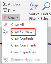
• In the Excel ribbon, navigate to the Home tab and click Clear.

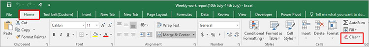
• Then, select the Clear Formats option.

The above steps will remove all unnecessary formatting from the selected cells, thus reducing the number of cell formats. Besides this, you can try removing the cell patterns (if any) or use cell styles  to remove unnecessary formatting in the workbook.

Method 2: Remove Conditional Formatting

Conditional formatting is also one of the reasons behind the “Too many different cell formats” error. It usually occurs if you have applied multiple rules to various cells or cell ranges within a workbook. Each rule has its own formatting settings. If you’ve applied a large number of conditional formatting to cells, it can increase the number of unique cell formats. You can check and remove the unnecessary conditional formatting. Here are the steps to do this:

• Open the Excel file in which you are getting the error.
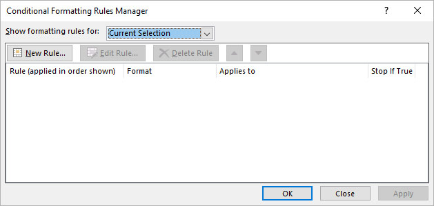
• Go to the Home tab and locate Conditional Formatting.

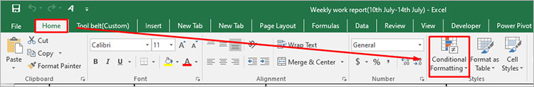
• Select Manage Rules.

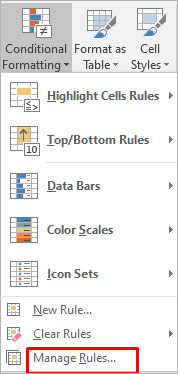
• The Conditional Formatting Rules Manager wizard is displayed. You can check the formatting rules and delete the unnecessary rule by clicking on the Delete Rule option.

Method 3: Repair your Excel Workbook

Corruption in the Excel workbook can also cause the “Too many different cell formats” error. You can try the Microsoft inbuilt utility to repair the file. Follow these steps to use this utility:

• Open your Excel application. Go to File > Open.
• Click Browse to choose the affected workbook.
• The Open dialog box will appear. Click on the corrupted file.
• Click the arrow next to the Open button and then select Open and Repair.
• You will see a dialog box with three buttons - Repair, Extract Data, and Cancel.

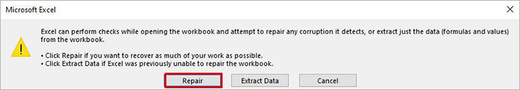
• Click on the Repair button to recover as much of the data as possible.
• After repair, a message is displayed. Click Close.

If the Open and Repair utility does not work or fails to repair the corrupted Excel file due to any reason, then you can use Stellar Repair for Excel to repair the Excel file. It is a simple-to-use third-party Excel repair tool with an intuitive UI that enables anyone to use it without much effort. The tool can help in fixing the “Too many different cell formats” error. It does so by repairing the Excel (XLS/XLSX) file and recovering all the components, including damaged cell style, without impacting the original formatting. You can download the software’s demo version and install it to check how it works.

Method 4: Save the Excel File to a Binary Workbook (.xlsb) Format

You can also get the “excel too many cell formats” error if the size of the spreadsheet is too large. You can try saving the Excel file in binary (.xlsb) format to reduce the Excel file size. Here’s how to do so:

• In Excel, navigate to File > Save As.
• Select Excel Binary Workbook (*.xlsb) in the Save as type dialog box.

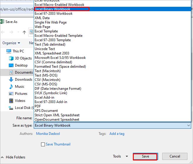
• Click Save.

Some Additional Solutions

Here are some additional methods you can try to fix the issue:

1. Check and Fix the Un-used Style Copy Issue

Many users have reported encountering the “Too many different cell formats” error when moving or copying the content of a workbook from one Excel to another and the unused styles being copied from one workbook to another. Microsoft has released a hotfix package which contains a fix for this issue. You can install this hotfix package (2598143 ) to resolve the issue.

2. Use Clean Excel Cell Formatting Option

You can check and enable the Excel cell formatting option to fix the “Too many cell formats” issue. This option will help you remove the excess formatting  in your workbook. To locate this option, click on the Inquiabove steps willre tab. If you fail to see the Inquire tab, then check if the Inquire option is enabled in the Excel Com Add-ins settings.

3. Clean up Workbooks using Third-Party Tools

The “Too many different cell formats” issue can occur if your workbook contains a large number of unnecessary styles, as mentioned above. You can use third-party tools, such as XLStyles Tool   or Remove Styles Add-in  to clean up workbooks recommended in Microsoft Guide. However, Microsoft takes no guarantee of these tools.

Closure

If you’re getting the “Too many different cell formats” error in Excel, try the methods discussed in this post to resolve it. You can simplify the formatting by following standardized guidelines and clearing all the unnecessary conditional formatting. If the error has occurred due to corruption in Excel file, then you can use Stellar Repair for Excel to repair the Excel file. It is an advanced tool that can repair Excel worksheet and recover all its objects without losing the original formatting.

How to Fix “File Not Loaded Completely” Error in Excel?

Summary: You may get the “File not loaded completely” error when opening a large-sized Excel file. Read this post to understand the causes behind this issue and the troubleshooting solutions to fix this Excel error. Also, you’ll get to know about an Excel repair tool that can help fix the issue if the cause is corruption in the Excel file.

Several users have reported experiencing the “File not loaded completely” error while opening Excel spreadsheets or when importing CSV file into Excel. This error can occur if the worksheet has crossed the maximum rows and columns limit , i.e., 1048576 rows by 16,386 columns. However, this issue can also occur due to various other reasons. Let’s take a look at the possible causes behind this error.

Why this Error Occurs?

The “File not loaded completely” issue can occur due to one of the following reasons:

• The Excel file you are trying to open is corrupted.
• The Excel file is too large.
• The Excel file has crossed the rows limit.
• Memory issue in your system.

Methods to Resolve the “File not Loaded Completely” Error

Following are some methods you can try to fix the Excel file not loaded completely issue.

Method 1: Try to Import the Spreadsheet into MS Access

A large-sized Excel file takes time and memory to load. When you try opening a large file, you may get the “file not loaded completely” error. It indicates your file contains unwanted rows and columns. In such a case, you can try importing your spreadsheet into Access. By doing this, you can easily access the rows and columns in the database table, and then remove the extra rows. Follow the steps below to import your spreadsheet into Access:

• Open a blank database in Access application.
• Navigate to the External Data tab and then click on the Excel button.

• In the Get Data-Excel Spreadsheet window, click Browse.

• In the File Open dialog box, select the Excel file (in which you are getting the error) and click Open.

• Select Import the source data into a new table in the current database and click OK.

• In the Import Spreadsheet Wizard window, you’ll see all the rows and columns of your Excel file. Click Next.

• In the dialog box that appears, you can modify the field information (extra columns or rows).

• Once you performed the changes, click on the Next button.

• Provide a name to the table.

• Next, select the option “I would like a wizard to analyze my table after importing the data” (if you want to analyze the data) and click Finish.
• You will get a dialog box with a message. Click Yes.
  
• The Table Analyzer wizard will appear on the screen.

• Click on the Next button.

• Follow the instructions of the Table Analyzer wizard.
• Once you complete all the steps, select “Save import step” and click Close.

Method 2: Split Your Large Excel File

You may face the Excel file not loaded completely issue when importing a large Excel file. In such a case, you can try splitting your large file into smaller ones. To split the file, you can use VBA codes or the move or copy feature.

Method 3: Stop Unwanted Processes Running in the Background

Sometimes, you get the “File not loaded completely” error if you are running multiple files or programs simultaneously. You can check and stop unnecessary background processes in Windows using your system’s Task Manager. Here are the steps:

• Press the Ctrl+Shift+Esc keys to open the Task Manager window.

• Navigate to the Processes tab and check the Memory section.
• You can see the memory consumption of all the applications in your system.
• Select the unwanted applications and click on End Task.

Now, try to open the Excel file.

Method 4: Repair your Excel File

Sometimes, Excel throws the “File not loaded completely” error if it fails to read the data in your file. This might happen if your Excel file is corrupt. You can use the Open and Repair utility in Excel to repair your Excel file. Follow the below steps:

• In Excel, click the File tab and then click Open.
• Click Browse to select the desired file.
• In the Open dialog box, click on the corrupted file.
• Click on the arrow next to the Open button and then select Open and Repair.

•  Click on the Repair button.

• After repair, you will see a message as shown in the below figure.

• Click Close.

An Alternative Solution

If your file gets corrupted, then repairing it using the “Open and Repair” utility is a good option. However, the Open and Repair utility may not work if the file is severely damaged or corrupted. In such a case, you can use a professional Excel repair tool, such as Stellar Repair for Excel. This tool is primarily designed to repair inaccessible or corrupted Excel files. It can effectively work even if your file is too large or severely damaged. It can recover all the data from the corrupted Excel file without impacting its actual format. The software supports Excel files of almost all Excel versions.

Conclusion

The File not loaded completely issue in Excel may occur due to numerous reasons. Try the troubleshooting methods listed above to resolve the issue. If the Excel file is corrupt, then you can try repairing your file using the Open and Repair tool. However, it can fix only minor corruption issues. If your file is severely corrupted, then use Stellar Repair for Excel . The software offers you the safest way to repair your Excel file without making any changes in the formatting. You can download the free trial version of the software today to scan and preview the Excel file.

Also read: